The simplest thing that can be simulated with the mechanics simulation patch is the movement of individual point masses. Their movement under the influence of gravity and environment objects is handled in this part.

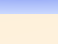
We start with a simple scene setup:

To simulate the movement of a single mass we add the following to the global_settings{}:

mechsim {		
  gravity <0, 0, -9.81>
  method 1

  environment {
    object plane { z, 0 }
    damping 0.9
    friction 0.1
    method 2
  }

  time_step (1/30)/300
  step_count 300
		
  #if (frame_number=1)
    topology {
      mass { <-2.8, -8.0, 0.9>, <2, 5, 0>, 0.1 density 5000 }
      save_file "tut02.dat"
    }
  #else
    topology {
      load_file "tut02.dat"
      save_file "tut02.dat"
    }
  #end
}

The purpose of the individual lines of this block is the following:

gravity <0, 0, -9.81> activates a standard gravity force in negative vertical direction.

method 1 selects simulation method 1 (Euler integration).

The environment {} block contains the definition of the environment. It contains:

The next two lines specify the timing of the simulation:

Finding the right step size is probably something most difficult for the beginner. A smaller step size generally leads to more accurate results. Usually the step size has to be below a certain value depending on the other simulation settings to get usable results, but it is not always obvious if some strange result is due to large time steps. High stiffness values in environments, collision and connections usually require smaller time steps. If you experience unexpected results it is often worth trying to decrease the step size and see if problems vanish.

There is also the possibility to use adaptive time stepping that will be introduced in the next part of this tutorial.

What follows is an #if conditional. It makes sure the mass is generated in the first frame and saved to the file while the following frames load and save the simulation data.

The first part contains statements for the first frame:

The topology{} block contains a singular mass{} section. It contains:

The save_file statement finally saves this mass to a file.

The second part contains the variant for the subsequent frames.

The topology{} block here contains just load_file and save_file statements referring to the same file. This makes MegaPOV load the old simulation data at the beginning, calculate the steps for the current frame and save to the same file afterwards.

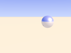
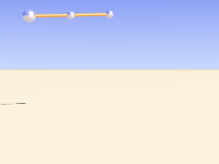
To show the mass in the scene we can use a macro from the mechsim.inc include file:

#include "mechsim.inc"

MechSim_Show_All_Objects(-1, false, -1, "")

The meaning of the parameters of this macro is described in Section 3.4.4.2, “MechSim_Show_All_Objects()”.

Now all we need to do is render the scene using the render options that can be found in the scene file comment and we get the following result:

In the first part of the tutorial we have handled masses and their movement under the influence of gravity and the constraints of the environment. If several masses exist in the simulation collisions between have to be taken into account.

For turning collision calculation on the following block is added to the mechsim{} section:

collision {
  1, 0, 0
  stiffness 60000
  damping 4000
}

The first three numbers tell MegaPOV which collision to calculate. For details see Section 2.7.4.1.3, “The collision settings”. The numbers used here turn calculation on for all mass-mass collisions.

stiffness (unit kg/s²) and damping (unit kg/s) influence how the masses interact.

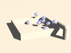
Another change made in this tutorial step is changing the environment to function based calculations. This usually leads to more accurate environment collisions, especially with more complex geometries.

Defining the environment as a function is fairy easy with the IsoCSG library. The definition in this case looks like:

#include "iso_csg.inc"

#declare fn_Env=
IC_Merge5(
  IC_Plane(z, 0),
  IC_Box(< 1.7,-1.7,-1.0>, < 1.5,1.7,0.5>),
  IC_Box(<-1.7,-1.7,-1.0>, <-1.5,1.7,0.5>),
  IC_Box(<-1.7, 1.7,-1.0>, <1.7, 1.5,0.5>),
  IC_Box(<-1.7,-1.7,-1.0>, <1.7,-1.5,0.5>)
)

Note that the stiffness, damping and friction parameters in the environment now have the same meaning as in the collision settings because it uses calculation method 1 (force based environment collisions).

Force based environment collisions lead to a more realistic simulation of the interaction of the masses with the environment since the movement of the masses does not abruptly change. Using this method is necessary for all higher order integration methods which will be introduced later.

This scene also adds new masses during the animation. This is achieved by adding the following code to the topology{} section:

#if (mod(frame_number, 6)=5)
  mass { < 1.3,-1.55,0.8>, <-0.2, 5, 0>, 0.18 density 5000 }
#end

It means that in every sixth frame a new mass is added at the starting position with the same starting velocity as the first mass.

Apart from masses there is another important element that can be added to the topology{} section: connections. Connections can be seen as springs. They connect two point masses and exert a force on them depending on the current distance of the masses compared to the relaxed length of the connection. In addition there is a damping property generating dissipative forces.

A connection{} block is added to the topology{} section like a mass:

connection { 0, 1 stiffness 50000 damping 2000 }

It contains:

if no length is given the current distance of the masses is used.

The mass indices are counted in order of creation starting at zero. The three connected masses from the following scene are created with:

topology {
  mass { <0, 0, 2.4>, <0, 0, 0>, 0.1 density 5000 fixed on }
  mass { <1, 0, 2.4>, <0, 0, 0>, 0.1 density 5000 }
  mass { <2, 0, 2.4>, <0, 0, 0.6>, 0.15 density 5000 }
  connection { 0, 1 stiffness 50000 damping 2000 }
  connection { 1, 2 stiffness 50000 damping 2000 }
}

The fixed on in the first mass definition fixes the position of this mass.

With plenty of such connections we can form more complex shapes. The mechsim.inc include file (see Section 3.4, “The 'mechsim.inc' include file”) contains several macros forming grids of masses and connections.

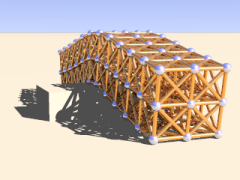
Placing the following in the topology{} section generates a box-like grid of connected masses:

MechSim_Generate_Block(
  <0, 0, 0>, 0.07, 1500, 22000, 2000, true,
  <-0.5, -2.75, 1.0>, <0.5, 2.75, 2.0>, <3, 12, 3>, No_Trans, 3
)

The meaning of the different parameters is described in Section 3.4.5.11, “MechSim_Generate_Block()”.

Apart from the grid macro we introduce a different simulation method in this scene. method 3 uses adaptive time stepping. This means you don't need to specify a step size but instead specify how accurate the simulation should be. The accuracy option takes two parameters: the maximum allowed local discretization error and the minimum step size to use.

Note that you might still need to specify an appropriate starting step size using time_step - the default value might not be appropriate.

In addition to the accuracy settings the total time per frame is specified using the time parameter.

The resulting animation shows a moving and deforming box geometry.

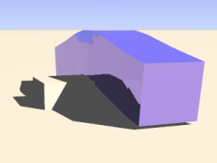
The MechSim_Generate_Block() macro also generates faces for the outside surface of the box. Faces are triangles each connecting three masses. They can be used for collision calculations and for displaying the geometry as a mesh. The latter can be done easily by changing the parameters of the MechSim_Show_All_Objects() macro:

MechSim_Show_All_Objects(-1, true, -1, "")

Apart from 3D grids we of course can also create 2D rectangular patches. Such objects behave like cloth or foil and offer a very interesting field of simulation.

Like 3D grids rectangular patches can be created with macros from the mechsim.inc include file (see Section 3.4, “The 'mechsim.inc' include file”):

MechSim_Generate_Patch_Std(
  <0, 0, 0>, 0.03, 8000, 10000, 0,
  true, <0.055, 0.055>, <50, 50>, Trans1, 2
)

This creates a 50x50 masses patch, again movable with a transform. Description of the parameters can be found in Section 3.4.5.15, “MechSim_Generate_Patch_Std()”.

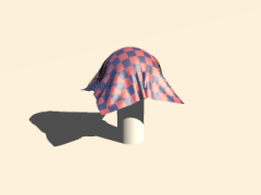
The following sample scene also uses a different simulation method than the previous scenes. It is called gradient descent method. It does not integrate the equations of movement like the other methods but moves the masses directly according to the forces influencing them. Inertia does not have effect with these method, therefore oscillations can't occur. Still the step size has to be chosen small enough for accurate results. The movement won't look very realistic in an animation but the final result can be used for a still render. Another disadvantage is the lack of friction, therefore the patch slides off the sphere in the end.

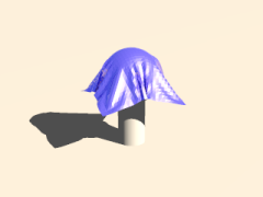
There is also a specialized macro for generating a mesh from a patch topology including normal vectors and uv coordinates. Rendering the previous topology with this macro results in the following picture:

There are a lot more aspects of the mechanics simulation patch that are not handled in this tutorial yet. Reading the reference (see Section 2.7.4, “Mechanics simulation patch”) and mechsim.inc include file documentation (see Section 3.4, “The 'mechsim.inc' include file”) should help learning about those things. The sample scenes show several examples what the simulation system can be used for but there are a lot more possibilities.

Masses can not only collide but also can interact in a freely definable way. This way you can simulate physical effect like electromagnetic fields and gravity.

Mass interaction is defined globally with theinteraction keyword in the mechsim{} block. For the inverse square law of gravity you for example could use the following setup:

// Gravitation constant: 6.672e-11 m^3*kg^-1*s^-2
#declare G=6.672e-11;

// Newton's law of gravitation
#declare fn_Gravity=
  function(x, y, z, dist, m1, m2) {
    (G*m1*m2)/(dist*dist)
  }

global_settings {
  mechsim {
    ...
    interaction {
      function(x, y, z, dist, m1, m2) { fn_Gravity(x, y, z, dist, m1, m2) }
    }
    ...
  }
}

As you can see the interaction function has 6 parameters. The first three are the usual coordinates so you can define an interactions that differs depending on the absolute position. The last three are optional, the first of them is the distance between the masses and the other two the masses of the two masses that interact.

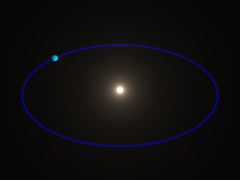
The simulation system calls this function for every pair of masses in every simulation step. This can of course be quite slow with a lot of masses. But in this simple example we only want to simulate the movement of the earth around the sun which is done with the following topology definition:

#declare Mio_km=1.0e9;

topology {
  // Sun
  mass { <0,0,0>, <0,0,0>, 696.0e6 mass 1.99e30 }
  // Earth
  mass { <149.6*Mio_km,0,0>, <0,29.8*1000,0>, (6371.0)*1000 mass 5.97e24 }

  save_file "tut09.dat"
}

Simulating this with 1 step per day is done with the following code:

step_count 2000

// 1 day per step
time_step (24*3600)/2000

topology {
  load_file "tut09.dat"
  save_file "tut09.dat"
}

And results in the following movement. The size of the sun and earth is of course strongly exaggerated. You can find a more complex simulation of all the inner planets in the planets.pov sample scene.