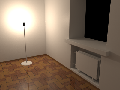
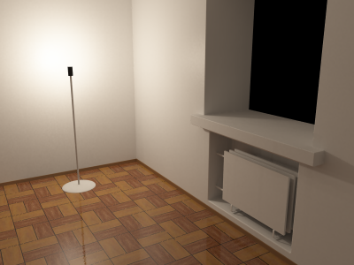
This addition simulates decrease of reactive chemicals in film emulsion during exposure. The areas that have received more light react less than other areas. Useful for high contrast scenes as it brings up the dark areas and limit bright areas.
There are two new keywords in the global_settings block:
exposure FLOAT
exposure_gain FLOAT
where exposure_gain is optional and has default value 1. Both parameters have to be greater than 0 to influence rendering.
exposure can be thought as film speed, aperture and exposure time multiplied together. The value is not absolute. If the light source intensities in the scene are multiplied by 10 and exposure value is divided by 10 the resulting image will be the same.
exposure_gain can be used to brighten scenes with low maximum intensity when also low exposure value is used.
The equation for such behavior of color used in MegaPOV is:
color = exposure_gain * (1 - exp( - exposure * color )).
Example 2.11. Various values for film exposure simulations
Examples which map range 0-1 to range 0-1 with increasing amount of compression:
exposure 0.05 exposure_gain 20   // almost linear
exposure 0.2  exposure_gain 5.5
exposure 0.5  exposure_gain 2.5
exposure 1    exposure_gain 1.6
exposure 10   exposure_gain 1
exposure 100  exposure_gain 1    // high compression
Traditionally the color values POV-Ray™ calculates for the image pixels were clipped right at the beginning, before calculating the antialiasing. Further color processing was not done (except gamma correction). In POV-Ray™ 3.6.1 clipping was moved to be applied after antialiasing which also made it unnecessary to turn it off explicitly for high dynamic range image output. But in a lot of cases this is not the optimal solution for high quality antialiasing.
This patch offers a way to specify a custom tone mapping function for both before and after antialiasing. This way you can for example apply the pre-aa clipping known from POV-Ray™ 3.5 or an exponential exposure curve like in the film exposure simulation patch (see Section 2.7.1, “Film exposure simulation”).
By also allowing to specify a mapping function after antialiasing you can also invert the mapping used and get back the linear color values. The antialiasing in this case is aimed at the used mapping function and when a similar function is applied in an imaging program afterwards the antialiasing will look good. The patch also offers automatic numerical inversion of the mapping function.
The syntax is:
global_settings {
  tone_mapping {
    function { FUNCTION_ITEMS }
    [inverse INTEGER | function { FUNCTION_ITEMS }]
  }
}
The functions are user defined float functions with at least one parameter. The original color value is passed as the first parameter and the return value specifies the resulting color. Using
function { min(1, x) }will for example result is a simple clipping.
Specifying an integer value instead of a user defined function after inverse makes MegaPOV numerically invert the function with the number of sample points specified. For non-invertible functions this might lead to unexpected results.
Example 2.12. Exponential tone mapping
The following code applies an exponential exposure curve like the film exposure simulation patch:
#declare Exposure=1.6;
#declare Exposure_Gain=1.0;

global_settings {
  ...
  tone_mapping {
    function { Exposure_Gain - exp( -Exposure * x ) * Exposure_Gain }
  }
}
The include file tone_mapping.inc coming with MegaPOV offers several macros with useful tone mapping functions (see (see Section 3.6, “The 'tone_mapping.inc' include file”));
In POV-Ray™ 3.5 and earlier temporary files with cache of radiosity were named the same for every frame in the animation rendering. Since MegaPOV 1.0 the name of this file is concatenated from the name of the currently rendered image. Together with Frame_Step (see Section 2.1.1, “Frame_Step”) and this addition it is finally possible to start two parallel processes with radiosity rendering over one source.
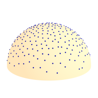
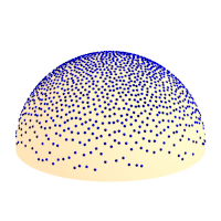
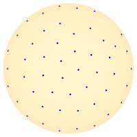
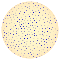
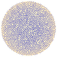
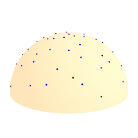
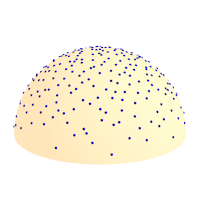
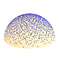
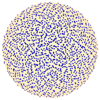
The radiosity function in POV-Ray™ 3.5 uses an internal table of directions for the rays that are traced from a sampling point to determine the irradiance at that point. This patch allows to select alternative sets of sample ray directions. This can help both to overcome the limit for maximum count of 1600 as well as improve the quality of results at lower count values.
The syntax description of this feature is:
RADIOSITY_ITEMS:
    ...
    [ samples SAMPLES_ITEMS ]

SAMPLES_ITEMS:
    INT_SAMPLES_TYPE |
    {
      SAMPLES_COUNT,
      VECTOR_DIRECTION, ...
      [weight INT_WEIGHT_TYPE]
    }
MegaPOV contains an internal generator for sample direction using the halton sequence written by . It is activated by adding:
samples 1
to the radiosity{} block. The default value (0) uses the old internal direction table.

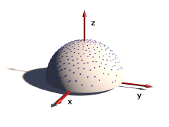
The sample ray directions can also be defined directly in the scene file:
samples {
  300, // number of directions given
  <0.78080, -0.36618, 0.50622>,
  <-0.26409, -0.01064, 0.96444>,
  ...
}
A number of sample direction sets is coming with MegaPOV as include files.
The coordinate system for these sample ray directions is relative to the surface at the sample position. The z-Axis points in normal direction. All directions should be in the upper hemisphere (z coordinate >0).
An optional weight parameter allows to weight the sample intensity with cos(theta) where theta is the angle between the normal vector and the ray direction. The sample ray directions should have a density distribution according to this function. If a uniform distribution is used instead weight 1 would weight the sample rays to compensate this. The default is 0 which turns off special weighting.
This patch is based on an idea by . Normally the distribution of radiosity rays is identical for all sample points. This patch rotates the sample set around the vertical axis by a random angle for each sample taken. This can help to reduce artefacts in some cases.
This patch is activated the following way:
radiosity {
  ...
  randomize on
}
| Note | |
|---|---|
Since this feature uses a random number for the sample direction rotation it is not safe to use it in animations. Also a partial render of a scene will produce different results than rendering the whole scene. | |
The POV-Ray™ radiosity feature uses the error_bound parameter to decide when to reuse radiosity samples already in the cache and when to take a new sample because there are not enough samples nearby. Setting a low error_bound makes POV-Ray™ take a new sample very often and therefore leads to more accurate calculation of the diffuse illumination but at the same time is prone to artefacts when used with a low number of sample rays (count).
Especially with geometries containing sharp edges the sample density can become very high because POV-Ray™ recognizes the lighting changes very rapidly there. In such cases it will not be possible to take all required samples during pretrace which is unfortunate because it leads to slow renders, increasing memory requirements during the render and makes splitting the render into multiple tasks more difficult. POV-Ray™ already offers the always_sample option that reduces the necessity of additional samples in the final render pass by setting nearest_count to 1 on the final pass so only one sample is required per radiosity evaluation but this only reduces the problem a bit and is prone to artefacts.
The adaptive error_bound allows you to set a range the error_bound value is automatically chosen from as well as an overestimation factor used to find the optimal error_bound value. This means the radius from which cached radiosity samples are used is increased if not enough samples are found in the area defined by the original error_bound. In a way this is similar to the adaptive search radius used in photon mapping.
This patch is activated by using the following syntax instead of the standard error_bound parameter:
RADIOSITY_ITEMS:
    ...
    [ error_bound ERROR_BOUND_DEFINITION ]

ERROR_BOUND_DEFINITION:
    FLOAT_ERROR_BOUND |
    {
      FLOAT_ERROR_BOUND
      [adaptive FLOAT_EB_OVERESTIMATION [, FLOAT_ERROR_BOUND_MAX] ]
    }
The default values are:
FLOAT_EB_OVERESTIMATION : 1.5
FLOAT_ERROR_BOUND_MAX : 10.0
The following code for example might be used for an adaptive error_bound:
radiosity {
  ...
  error_bound { 0.3 adaptive 2.0, 20 }
}
Note it can be necessary to use fairly large maximum values to avoid final pass radiosity samples to be necessary. The overestimation factor increases the render time when chosen too small and will result in unnecessarily large errors when very large. Values between 1.5 and 2 are usually a good choice.
The patch introduces some additional statistics showing the number of samples taken in pretrace and final pass and separately for the different recursion levels. This can be useful for optimizing the radiosity settings.
The purpose of the radiosity pretrace is to take care of an optimal distribution of radiosity samples in the scene. For achieving this the view area is sampled with increasing density until pretrace_end. During pretrace pass the error_bound is also reduced with low_error_factor. The results are usually quite good but this is unnecessarily slow in a lot of scenes where different areas require a very different sample density. Also the standard pretrace only samples down to a 2 pixel density which is not sufficient in many cases.
Because of these limitation practical use of radiosity usually does not take all radiosity samples during the pretrace. Sometimes it is even more efficient to totally avoid the pretrace.
This patch introduces a new pretrace mode which no more samples the whole view with the same density but adapts the sampling to the scene's requirements. To accomplish this the pretrace no more traces the different subdivision levels one after the other but subdivides the view in a recursive way.
In addition the new pretrace can also subdivide to a sub-pixel density (by using pretrace_end smaller than 1/image_width). This can of course be quite slow depending on the scene, render- and radiosity-settings.
The new pretrace is activated the following way:
radiosity {
  ...
  adaptive 1
}
The following values can be used for the radiosity parameter:
- 0 old pretrace, default.
- 1 new pretrace, subdivide until no new sample has to be taken.
- 2 new pretrace, one additional subdivision level in addition to 1.
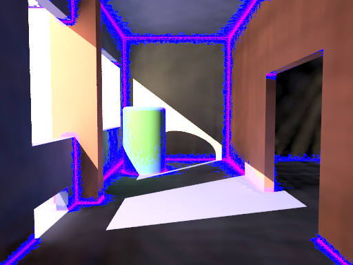
The POV-Ray™ radiosity code contains code to visualize the way radiosity works internally in the rendered images. This code is deactivated by default. This patch offers access to these features from SDL with some new parameters in the radiosity block.
The syntax of these parameters is the following:
RADIOSITY_ITEMS:
    ...
    [ show_samples FLOAT_RADIUS, COLOR ]
    [ show_low_count COLOR_LOW_COUNT, COLOR_GATHER_FINAL ]
The show_samples parameter activates the marking of the radiosity sample locations with the specified color. Note this color only sets the ambient value returned by the radiosity function. The other finish components are added to this. Therefore it might be necessary to use quite extreme color values for this. The radius parameter influences how large the sample spots are marked.
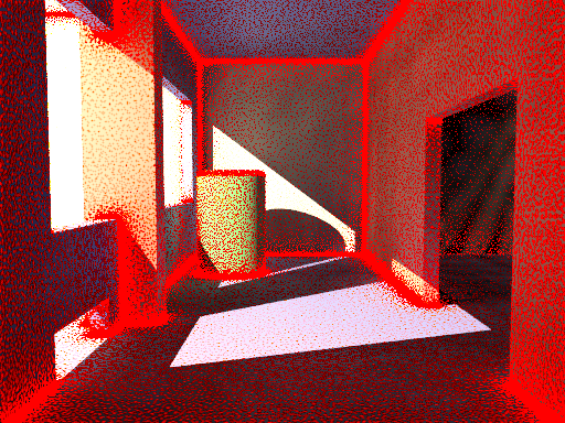
The show_low_count activates the marking of areas where the sample density is too low so less than nearest_count samples are available for the radiosity estimation. The color of these areas is chosen with the first parameter. This is only visible when always_sample is off, otherwise additional samples are taken in the final pass and the area is colored with the second color specified.
The mechanics simulation system is integrated into the POV-Ray™ rendering system. The simulation parameters are set in the global_settings{} block of the scene file. While parsing the scene MegaPOV calculates the simulation exactly where it occurs in the file. This way the simulation can interact with the scene by using objects, functions and values set before the mechsim{} block in the scene file. But additionally the simulation data can also be used in the scene later on for placing objects according to the simulation results.
This patch introduces a new block in the global_settings{} section of the POV-Ray™ scene file.
The complete syntax description of this block is:
MECHSIM:
    mechsim { [MECHSIM_ITEMS...] }
MECHSIM_ITEM:
    method INTEGER | bounding INTEGER |
    gravity VECTOR | time_step FLOAT |
    step_count INTEGER | time FLOAT |
    start_time FLOAT | end_time FLOAT |
    accuracy FLOAT[, FLOAT] |
    environment { ENVIRONMENT_DEFINITION [ENVIRONMENT_ITEMS...] } |
    interaction { INTERACTION_DEFINITION ... } |
    field { FIELD_DEFINITION ... } |
    force { FORCE_DEFINITION ... } |
    attach [VECTOR] { ATTACH_DEFINITION ... } |
    fixed VECTOR |
    collision { COLLISION_TOGGLE [COLLISION_ITEMS...] } |
    topology { [GROUP_DEFINITIONS...] [TOPOLOGY_ITEMS...]
               [save_file FILE_NAME [Type]] }
ENVIRONMENT_DEFINITION:
    function [(IDENT_LIST)] { FUNCTION_ITEMS } | object OBJECT
ENVIRONMENT_ITEM:
    stiffness FLOAT | damping FLOAT | friction FLOAT [, FLOAT] |
    method INTEGER
INTERACTION_DEFINITION:
    function [(IDENT_LIST)] { FUNCTION_ITEMS }
FIELD_DEFINITION:
    function { SPECIAL_COLOR_FUNCTION }
FORCE_DEFINITION:
    function { SPECIAL_COLOR_FUNCTION }
ATTACH_DEFINITION:
    function { SPLINE }
COLLISION_TOGGLE:
    [INT_MASS_MASS [, INT_MASS_FACE [, INT_CONNECTION_CONNECTION]]]
COLLISION_ITEM:
    stiffness FLOAT | damping FLOAT | friction FLOAT [, FLOAT]
GROUP_DEFINITION:
    group [(INT_GROUP_INDEX)] { TOPOLOGY_ITEMS... }
TOPOLOGY_ITEM:
    mass { V_POSITION, V_VELOCITY, F_RADIUS
           mass FLOAT | density FLOAT
           [attach INTEGER] [force INTEGER] [fixed BOOL] } |
    connection { INDEX1, INDEX2 [stiffness FLOAT] [damping FLOAT]
                 [length FLOAT] } |
    viscoelastic { INDEX1, INDEX2 [stiffness FLOAT] [length FLOAT]
                 [accuracy FLOAT] [ VE_ELEMENTS...  ] } |
    face { INDEX1, INDEX2, INDEX3 } |
    load_file FILE_NAME
VE_ELEMENT:
    element { F_STIFFNESS, F_DAMPING [, F_POSITION ] ] }
Some general parameters can be given in the top level of the mechsim{} section.
The default values are:
method : 1
bounding : 0
gravity : <0, 0, 0>
time_step : 0.1
step_count : 10
Selects the integration method used for solving the equations of movement.
Possible values are:
- 1 (MECHSIM_METHOD_EULER) simple forward Euler integration method
- 2 (MECHSIM_METHOD_HEUN) second order (Heun) integration method
- 3 (MECHSIM_METHOD_RUNGE_KUTTA) fourth order Runge Kutta integration method
- 4 (MECHSIM_METHOD_GRADIENT) gradient descent method
Method 1 is a first order integration method also known as explicit Euler method. With the differential equations of movement written as:
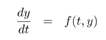 |
y being the state of the system (positions and velocities) and the initial conditions y(t0)=y0 the Euler method can be written as:
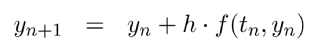 |
Method 2 is a second order integration method known as Heun's method. Its formula is:
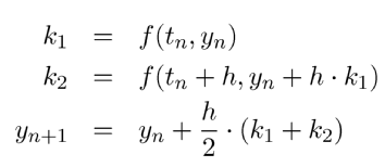 |
Method 3 is a fourth order integration method known as the classical Runge-Kutta method, in contrast to method 1 and 2 it automatically controls the time steps (see Section 2.7.4.1.1.6, “adaptive time stepping”):
 |
Selects the bounding method to speed up collision detections between masses, connections and faces.
Possible values are:
- 0 (MECHSIM_COLLISION_BOUNDING_NO) no bounding system
- 1 (MECHSIM_COLLISION_BOUNDING_AUTO) automatically select method 0, 2 or 3 depending on complexity
- 2 (MECHSIM_COLLISION_BOUNDING_BOX) speed up using bounding boxes
- 3 (MECHSIM_COLLISION_BOUNDING_HASH) speed up using spatial hashing
The bounding techniques have been implemented by .
Applies an overall constant gravitational force to all masses.
A vector is expected, the unit is m/s².
Standard earth gravity (with y=up coordinates) is:
gravity <0, -9.81, 0>
With field functions (see Section 2.7.4.1.6, “Field forces”) non constant gravity can be simulated
All movements in the simulation system can be fixed in one or two directions using the fixed option.
This can be used to make the MechSim system perform simulation of 2D and 1D systems. Note however that the simulation still runs in 3D internally.
by adding:
fixed <0, 0, 1>
to the mechsim{} block you can for example perform a simulation in the x-y-plane.
All simulation methods use discrete time steps for calculating the simulation. There are three parameters to steer this but only two are needed to correctly define the stepping. The formula for calculating the third is:
Step_Count = Time / Time_Step
An optional start_time value allows to specify a starting time different from 0. Changing this can influence the attach and environment function. (see Section 2.7.4.1.7, “Attaching masses” and Section 2.7.4.1.2, “The environments”) Specifying an end_time value instead of time is also possible.
| Important | |
|---|---|
Using too large time steps can lead to instability in the simulation. MegaPOV will recognize this in most cases and stop simulation with an error message but this does not mean the simulation is correct as long as no error is reported. Simulation results should always be checked for plausibility. | |
Simulation method 3 automatically controls the used time steps. This is done by calculating every step with double steps size and comparing the results. So the local discretization error is automatically kept below a specified threshold. You can specify this threshold and the minimum allowed step size with the accuracy keyword:
accuracy THRESHOLD, MIN_STEP
the minimum step size is optional, default values are:
THRESHOLD : 1.0e-5
MIN_STEP : 1.0e-7
The step size to start with can be specified with time_step. It is usually not critical but can be necessary to be set sufficiently low for a successful simulation.
The render statistics show the actual minimum, average and maximum time steps used during the simulation.
Example 2.13. Adaptive time stepping
A simulation setup for adaptive time stepping could look like:
mechsim {
  ...
  method 3
  time 1/30
  accuracy 1e-5, 1e-6
  ...
}
| Note | |
|---|---|
Adaptive time stepping guarantees a certain local accuracy of the simulation, it does not prevent instability though. It will not be possible to simulate a system that does not run with fixed time steps. | |
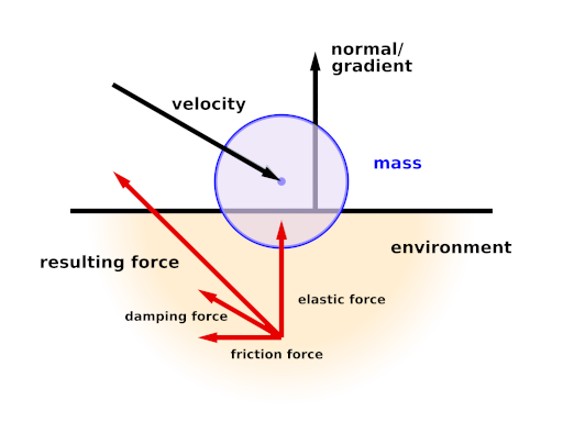
Environments are shapes the simulated masses are supposed to interact with. Several of them can be created with environment{} blocks.
An environment is defined either by a user defined function or an object. If both are given the function is preferred.
Apart from the default parameters (x, y and z) the function can have a fourth parameter supplying a time index. This way moving environment objects can be simulated.
#declare fn_Env=function(x, y, z, tim) { z-tim }

global_settings {
  ...
  mechsim {
    ...
    environment {
      function(x, y, z, tim) { fn_Env(x, y, z, tim) }
      ...
    }
  }
}
There are three parameters defining the properties of the environment:
stiffness The elasticity parameter of the surface. The unit is N/m or kg/s².
damping Depending on the environment calculation method (see below) this is either a diminishing factor (<1) applied to the mass velocities at each collision or a damping constant (unit kg/s)
friction The friction factor controls the amount of friction during collisions. An optional second parameter, the friction excess value should usually be slightly larger than 1 and causes the friction to occur already slightly above the surface. This can be helpful to obtain realistic results.
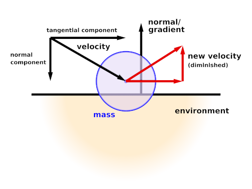
There are currently two methods how the environment collisions can be calculated:
Method 1 (MECHSIM_ENV_METHOD_FORCE) is force based. When a mass collides with the environment a force is applied in direction of the function gradient (with function based environments) or the surface normal (with objects). The stiffness, damping and friction parameters influence this force. friction defines the ratio between the tangential force and the normal force.
Method 2 (MECHSIM_ENV_METHOD_IMPACT) is based on impact laws. The velocity is inverted at the surface and diminished by the damping factor in normal direction and by the friction value in tangential direction. stiffness does not have any influence in this case.
Since this method directly modifies the velocity rather than applying forces it should only be used with the first order (Euler) integration method.
With the gradient descent simulation method the method parameter does not have any effect.
The collisions referred to here are not environment collisions but collisions between the simulation elements. Since detecting this kind of collision is quite computationally intensive it is turned off by default.
With three numbers at the beginning of the collision{} section collision can be toggled for mass-mass-collisions, mass-face-collisions and connection-connection-collisions. All these parameters are optional, the meaning of the possible values is:
- 0 (MECHSIM_COLLISION_NONE) No collisions of this kind are calculated.
- 1 (MECHSIM_COLLISION_ALL) Collisions between all simulation elements are calculated.
- 2 (MECHSIM_COLLISION_GROUP) Only collisions between elements of different groups are calculated.
Internal collisions are always calculated with forces. The same three parameters like in the environment settings can be used to specify the properties
- stiffness The elasticity parameter of the surface. The unit is N/m or kg/s².
- damping A damping constant (unit kg/s)
- friction The friction factor controls the amount of friction during collisions. An optional second parameter, the friction excess value should usually be slightly larger than 1 and causes the friction to occur already slightly before the collision. This can be helpful to obtain realistic results.
Example 2.14. An example for a complete collision{} section:
global_settings {
  ...
  mechsim {
    ...
    collision {
      2, /* mass-mass collisions between elements of different groups */
      0, /* no mass-face collisions */
      0  /* no connection-connection collisions */
      stiffness 20000
      damping 4000
      friction 0.2, 1.01
    }
  }
}
The topology{} section is the central part of the whole simulation settings. Here the simulation elements, their positions and properties, can be defined.
There are three topology items: masses, connections and faces. Each of them has several parameters that can be set.
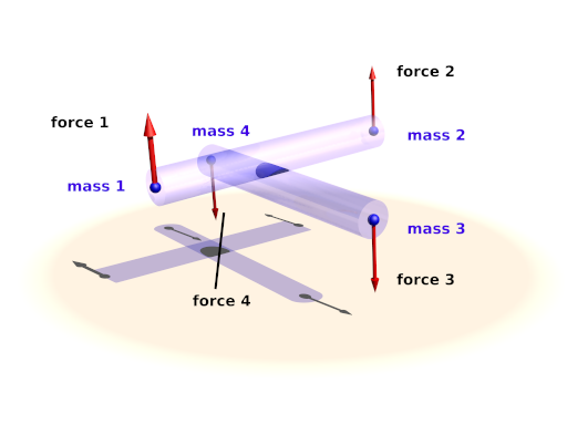
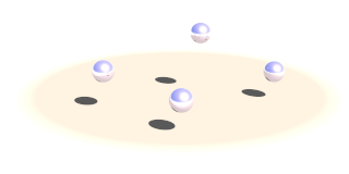
The mass block defines a point mass. These are the central elements of the simulation. Their movement is calculated by the simulation system.
The mass block contains the following elements:
- The first item is a vector specifying the position of them mass (unit: m).
- The second item, also a vector, represents the velocity of them mass (unit: m/s).
- The third item is a float standing for the radius of the mass (unit: m). This radius is only used in collision calculations (see Section 2.7.4.1.3, “The collision settings”). Otherwise the mass behaves as a point mass.
In addition either the mass (unit: kg) or the density (unit: kg/m³) of the element has to be given. If density is specified the resulting mass is calculated automatically. An optional boolean parameter (fixed) prevents the mass from moving if set to true.
A complete example for a mass definition:
mass {
  <0, 0, 1>, /* position */
  <1, 0, 0>, /* velocity */
  0.1        /* radius */
  density 600
  // mass 2
  // fixed true
}
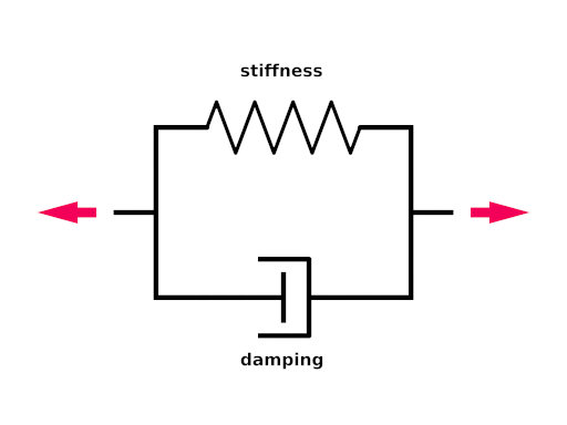
The connection block defines a connection between two point masses. It can have elastic and dissipative properties.
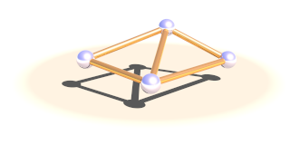
The first two elements of this block are integer numbers specifying the indices of the masses to connect.
Connections simulate a parallel elasticity and linear damping element - a so called Voigt-Kelvin-Element.
The force they exhibit on the masses they connect is:
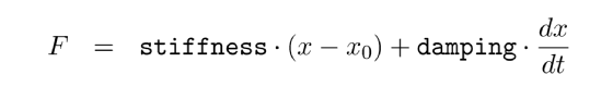 |
There are three optional parameters: The stiffness value specifies the elasticity of the connection (unit N/m or kg/s²). damping the velocity proportional damping factor (unit kg/s). The default value for both of these is zero. The third parameter allows to specify a relaxed length (x0) of the connection. If it is not specified the distance of the two masses at the time the connection is created is used for this property.
A complete example for a connection definition:
global_settings {
  ...
  mechsim {
    ...
    topology {
      mass { ... }  /* mass with index 0 */
      mass { ... }  /* mass with index 1 */

      connection {
        0,          /* index of the first mass */
        1           /* index of the second mass */
        stiffness 10000
        damping 2000
        // length 0.5
      }
      ...
    }
  }
}
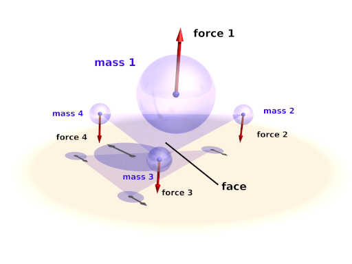
The face block defines a triangular face between three point masses. It is used for collision calculations (see Section 2.7.4.1.3, “The collision settings”) and can be useful for generating a mesh from the simulation data for display.
There are three integer numbers in the block, the indices of the masses forming the face.
A complete example for a face definition:
global_settings {
  ...
  mechsim {
    ...
    topology {
      mass { ... }  /* mass with index 0 */
      mass { ... }  /* mass with index 1 */
      mass { ... }  /* mass with index 2 */

      face {
        0,          /* index of the first mass */
        1,          /* index of the second mass */
        2           /* index of the third mass */
      }
      ...
    }
  }
}
Viscoelastic connections allow you to simulate more complex material properties than conventional connections. Conventional connections simulate a parallel elasticity and linear damping element - a so called Voigt-Kelvin-Element (see Section 2.7.4.1.4.2, “Connections”). With this element the force of the connection only depends on the momentaneous distance and velocity of the masses. Viscoelastic connections use a more complex model that also allows you to simulate effects like relaxation.
The element definition contains the index of the two masses it connects and a relaxed length - just like conventional connections. The stiffness value specifies the static elasticity of the connection (unit N/m or kg/s²). Furthermore you can specify an arbitrary number of parallel Maxwell-Elements. Each contains two mandatory parameters: the stiffness (unit N/m or kg/s²) and the damping (unit kg/s)
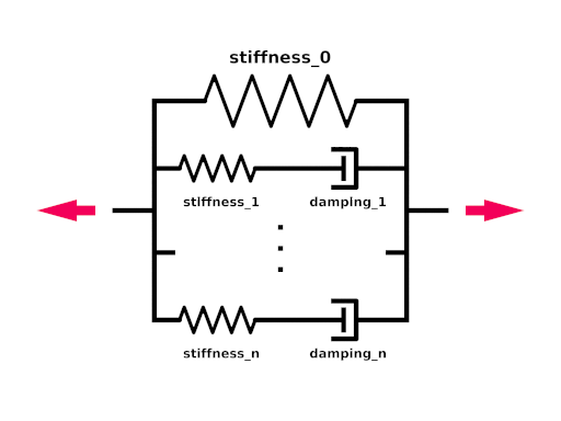
The force viscoelastic connections exhibit on the masses they connect is:
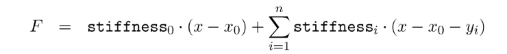 |
yi are the inner coordinates of the Maxwell-Elements that get calculated by the simulation system.
A complete example for a connection definition:
global_settings {
  ...
  mechsim {
    ...
    topology {
      mass { ... }       /* mass with index 0 */
      mass { ... }       /* mass with index 1 */

      viscoelastic {
        0,               /* index of the first mass */
        1                /* index of the second mass */
        stiffness 10000  /* static stiffness */
        element {        /* first maxwell element */
          2000,          /*   - stiffness */
          5000           /*   - damping */
        }
        element {        /* second maxwell element */
          4000,          /*   - stiffness */
          2000           /*   - damping */
        }
        // length 0.5
      }
      ...
    }
  }
}
| Note | |
|---|---|
In contrast to normal connections viscoelastic connections do not participate in collisions. If you want connection-connection collisions in your simulation you have to use normal connections in addition. | |
Simulation elements can be categorized into groups. The main purpose of this is to speed up collision tests. The group keyword can be followed by an integer number in parentheses to explicitly specify the group. Otherwise the group index is determined automatically.
global_settings {
  ...
  mechsim {
    ...
    topology {
      mass { ... }  /* these elements are group index 0 */
      ...
      group {
        mass { ... } /* these elements are group index 1 */
      }
      group {
        mass { ... } /* these elements are group index 2 */
      }
      group (1) {
        mass { ... } /* these elements are group index 1 */
      }

      ...
    }
  }
}
The topology data can be written to and loaded from files. For the format of these files see Section 2.7.4.3, “The simulation data file format”.
save_file can only be added to the main topology{} block. It saves the complete data after the simulation to the specified file.
load_file can be placed anywhere in the topology{} section. If placed in a group the elements in the file are added to that group. Otherwise they are are placed in groups according to group index information in the file.
The same file name can be specified for both loading and saving the data. This is especially useful for animation when the following frame simulation should start with the result of the last frame:
global_settings {
  ...
  mechsim {
    ...
    topology {
      load_file "mechsim_data.dat"
      save_file "mechsim_data.dat"
    }
  }
}
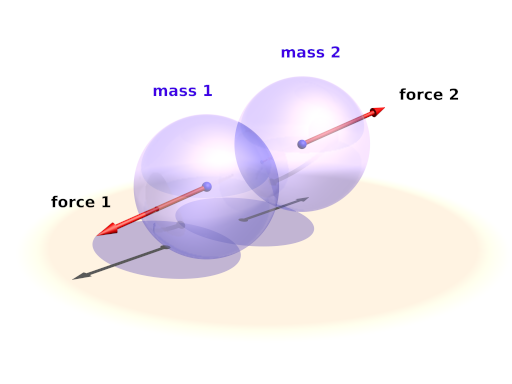
Masses can be set to exert forces on each other depending on the distance and the position in space. Phenomena like gravity in space and electrostatic fields can be simulated this way.
The interaction{} block can contain one or more user defined functions. Apart from the default parameters (x, y and z) the functions can have three additional parameters: the distance between the masses and the masses of the two masses that interact.
The function return value defines the force exerted on both masses in opposite directions. Positive values mean attractive forces and negative values repulsion.
To calculate the force on each mass the function is evaluated at the mass position for all combinations with other masses. The first mass parameter is always for the mass itself, the second is for the other mass interacting. In most cases the two mass parameters should be exchangeable in the formula of course.
General field like forces can be simulated using the field{} block. One example for such a field force is gravity although the simulation system has a special parameter for specifying such a simple constant gravity force. Much more complicated fields can be set up using this function.
The field{} block expects a pigment function defining the force components in the different directions. The red component of the pigment for the x direction, the green component for the y direction and blue for z. The mechsim include file (see Section 3.4, “The 'mechsim.inc' include file”) contains a macro generating an appropriate pigment function from three float functions.
Example 2.16. Constant downward force in Mechanics simulation
A function for a constant downward force (in y direction) would look like:
#include "mechsim.inc"

global_settings {
  ...
  mechsim {
    ...
    field {
      Vector_Function(
        function {0},
        function {-1},
        function {0}
      )
      ...
    }
  }
}
Note that in contrast to the gravity parameter the fields define a force and not an acceleration. Large masses will be influenced less than small masses.
Apart from adding the fixed flag to masses and thereby fixing them to a certain position we can also constrain them to a certain predefined movement. Those movements are described with spline functions in the attach{} block.
An optional vector can be added after the attach keyword to make the attachment only force the movement in one or two coordinate directions. Zero elements in the vector lead to free movement in that direction
Example 2.17. Attachment in Mechanics simulation
The following generates a linear movement in x direction, a constant position in y direction and a free movement in z-direction:
global_settings {
  ...
  mechsim {
    ...
    attach <1,1,0> {
      function {
        spline {
          linear_spline
            0.0, <0,0,0>
            0.5, <1,0,0>
            1.0, <2,0,0>
          }
        }
      }
      ...
    }
  }
}
These functions are automatically numbered starting from zero. To attach a mass to a function the attach parameter has to be set in the mass definition. The following mass is attached to the attach function with the number two:
mass {
  <0, 0, 1>, <0, 0, 0>, 0.1
  density 600
  attach 2
}
During the simulation the spline is evaluated at the current time value and the returned vector describes the movement of the attached masses. Note that the spline does not describe an absolute position for the masses, just their movement relative to their starting position. Attaching several masses to the same spline makes them perform a parallel movement.
The whole simulation data can be accessed anywhere in the POV-Script. This is achieved by adding new float/vector functions:
The complete syntax description of this block is:
FLOAT_FUNCTION:
    ... | mechsim : MECHSIM_ELEMENTS
MECHSIM_ELEMENTS:
    time | mass_count | connection_count | face_count |
    mass( INTEGER ) : MASS_FLOAT_ELEMENT |
    connection( INTEGER ) : CONNECTION_FLOAT_ELEMENT |
    viscoelastic( INTEGER ) : VISCOELASTIC_FLOAT_ELEMENT |
    face( INTEGER ) : FACE_FLOAT_ELEMENT
MASS_FLOAT_ELEMENT:
    radius | mass
CONNECTION_FLOAT_ELEMENT:
    index1 | index2 | length | stiffness | damping
VISCOELASTIC_FLOAT_ELEMENT:
    index1 | index2 | length | stiffness | accuracy | count |
    element( INTEGER ) : stiffness | damping | position
FACE_FLOAT_ELEMENT:
    index1 | index2 | index3

VECTOR_FUNCTION:
    ... | mechsim : MECHSIM_ELEMENTS
MECHSIM_ELEMENTS:
    mass( INTEGER ) : MASS_VECTOR_ELEMENT
MASS_VECTOR_ELEMENT:
    position | velocity | force
These elements correspond to those set in the mechsim{} block in global_settings{}. The mass position and velocity are the ones that are modified during simulation. The mass force is the summed force that accelerated the mass in the last simulation step. The mass_count connection_count and face_count values are especially useful inside the mechsim{} block to determine the current index:
global_settings {
  ...
  mechsim {
    ...
    topology {
      /* part 1 */
      mass { ... }
      mass { ... }
      connection { ... }
      ...

      #declare Start_Mass_Part2=mechsim:mass_count;
      #declare Start_Connection_Part2=mechsim:connection_count;

      /* part 2 */
      mass { ... }
      mass { ... }
      connection { ... }
      ...
    }
  }
}
The Start_Mass_Part2 and Start_Connection_Part2 variables can later be used to display the different parts of the simulation in different forms.
The time value returns the current time index of the simulation (in seconds). Inside the mechsim block this is the start time of the simulation, afterwards it returns the time index when the simulation ended.
The force values return the force a connection exerts on the masses it connects. This value is a scalar, the force is always in direction of the connection. Note this value can of course be calculated manually as well, it is supplied for convenience.
The file format used for storing the simulation data has changed in MegaPOV 1.2. Backwards compatibility is provided for reading MegaPOV 1.1 style simulation data files. The new file format is especially introduced for being forward compatible with future versions of MegaPOV. This means that data files written by newer versions of MegaPOV should still be possible to read with MegaPOV 1.2 - it will just ignore the data it cannot handle.
The file format - like the old one - is a ASCII text file format. It starts with a four character string ('MSIM') identifying the mechanics simulation file format. The second element (seperated by a comma) is an integer number specifying the subformat of the file. Subformat 4 is the current new format. Subformat 3 and lower are read with the backwards compatibility feature.
After that follows a line break and the first character of every line following indicates what kind of data is stored in that line. The following characters are recognized right now:
I: Info line - containing 4 number: the number of masses, connections, faces and viscoelastic connections in the file (all integer).
T: Timing line - containing 3 number: the current time index (float), the current time step size (float) and the number of steps (integer). If no timing parameters are specified in the mechsim{} block these are used. If adaptive time stepping is used the stored time step value is used as the starting time step.
M: Mass line (see Section 2.7.4.1.4.1, “Point masses”) - containing the following numbers:
- 3 numbers for the position (float vector), unit: m
- 3 numbers for the velocity (float vector), unit: m/s
- The mass (float), unit: kg
- The radius (float), unit: m
- A flag (integer) currently only containing the fixed value. This flag could contain other boolean values in the future (connected with logical OR) so it should be tested accordingly (if (flag & 1))
- The group index (integer)
- The attach index (integer) - -1 means not attached
C: Connection line (see Section 2.7.4.1.4.2, “Connections”) - containing the following numbers:
- The index of the first mass (integer)
- The index of the second mass (integer)
- The relaxed length (float), unit: m
- The stiffness (float), unit: N/m or kg/s²
- The damping constant (float), unit: kg/s
- The group index (integer)
F: Face line (see Section 2.7.4.1.4.3, “Faces”) - containing the following numbers:
- The index of the first mass (integer)
- The index of the second mass (integer)
- The index of the third mass (integer)
- The group index (integer)
V: Viscoelastic connection line (see Section 2.7.4.1.4.4, “Viscoelastic connections”) - containing the following numbers:
- The index of the first mass (integer)
- The index of the second mass (integer)
- The relaxed length (float), unit: m
- The static stiffness (float), unit: N/m or kg/s²
- The calculation accuracy (integer), 1 or larger
- The number of maxwell elements (integer)
For every maxwell elements: The value of the inner coordinate (float), unit: m, the stiffness (float), unit: N/m or kg/s²
and the damping (float), unit: kg/s.
Example 2.18. The simulation data file format
A short sample file looks like this:
MSIM, 4,
I 3 2 0
T 0.133333 0.00182897 16
M 0.000000000000 0.000000000000 2.400000000000 0.000000000000 0.000000000000 0.000000000000 20.944 0.1 1 0 -1 -1
M 0.998031324856 0.000000000000 2.309705370342 -0.078825113822 0.000000000000 -1.298327808122 20.944 0.1 0 0 -1 -1
M 1.996410451933 0.000000000000 2.390382496553 -0.094947075882 0.000000000000 -0.744192468433 70.6858 0.15 0 0 -1 -1
C 0 1 1 50000 2000 0
C 1 2 1 50000 2000 0
This file contains 3 masses and two normal connections between them. Simulation has progressed to 0.133333 seconds with a current time stepping of 0.00182897 and 16 steps per frame. The first mass is fixed, the others are moving freely.
Post processing allows manipulation of the color of the pixels after the rendering step is completed.
In the past, post processing of images required some third-party software (such as PhotoShop, Paint Shop Pro, or the GIMP) or older versions of MegaPOV that had implemented a few predefined effects.
MegaPOV 1.1 introduces a more generic approach to the post processing. Instead of being limited to a few predefined effects, access to the content of the rendered image through internal functions is now available for the user. By mixing these functions, any imaginable effect is possible. As an example of using these functions, some basic effects (in the form of macros) are provided with a similar syntax to the postprocessing effects included in older MegaPOV versions.
Post processing data is stored during rendering. This data contains several components: color of the pixel, intersection point, depth, normal - in other words all the information the raytracer receives for each of the pixels. For anti-aliased images only the data from the first ray is gathered. The storage is automatically turned on after the explicit call to one of predefined macros:
#version unofficial megapov 1.1;
#include "pprocess.inc"
// store data of the color and transparency
PP_Init_Alpha_Colors_Outputs()

// store data of the intersection point coordinates or <0,0,0>
PP_Init_IPoint_Outputs()

// store data of the normal at the intersection point or <0,0,0>
PP_Init_INormal_Outputs()

// store data of the perturbed normal at the intersection point or <0,0,0>
PP_Init_PNormal_Outputs()

// store the distance between camera and intersection point
PP_Init_Depth_Output()

// store the uv coordinates at the intersection point
PP_Init_UV_Outputs()

// allow access to intermediate post processing stages
// (color and transparency received from a previous post process stage)
PP_Init_PP_Alpha_Colors_Outputs()
| Important | |
|---|---|
When using post_process { }, do not forget to include the file "pprocess.inc" because this include file is needed to access the internal data. | |
| Note | |
|---|---|
If you do not need to store all the data mentioned in the macros listed above, you can pick one ore more of the dedicated internal functions mentioned further down. For example: store only the red component and the x coordinate of the intersection point for further usage. Check the content of the listed macros in the include file to find how to turn on only specific component storage. | |
Macros listed in the previous section enables internal functions with the following syntax:
// functions to access the color components and transparency
f_output_red(x,y)
f_output_green(x,y)
f_output_blue(x,y)
f_output_alpha(x,y)

// access to the intersection point coordinates
f_output_ipoint_x(x,y)
f_output_ipoint_y(x,y)
f_output_ipoint_z(x,y)

// access to the normal vector at the intersection point
f_output_inormal_x(x,y)
f_output_inormal_y(x,y)
f_output_inormal_z(x,y)

// access to the perturbed normal vector at the intersection point
f_output_pnormal_x(x,y)
f_output_pnormal_y(x,y)
f_output_pnormal_z(x,y)

// access to the distance between camera and intersection point
f_output_depth(x,y)

// access to the uv coordinates at the intersection point
f_output_u(x,y)
f_output_v(x,y)

// access to color and transparency of an earlier post processing stage
f_pp_red(x,y,Ref)
f_pp_green(x,y,Ref)
f_pp_blue(x,y,Ref)
f_pp_alpha(x,y,Ref)
The majority of the listed functions only need x and y parameters. These parameters are the location in the area of the rendered image. Not defined in pixels but in the range <0,1>.
Example 2.19. The internal post process function asking for red color at the middle of image
f_output_red(0.5,0.5)
Note that <0,0> is not the value of the most top-left pixel, but the value at the top left corner of the most top left _pixel_. You have to shift it about <0.5/image_width,0.5/image_size> to hit the center of the most top left pixel. If you are not happy with the need of expressing coordinates in decimal form you can always express them in relation to the image size.
Some of the functions contain an additional Ref parameter. These are functions which refer to the result of the earlier calculated post processing stage. This parameter specifies to which stage we refer: 0 means output of rendering, 1 means output of first post processing, 2 means output of second postprocessing, etc.
Numbering depends on the order of appearence in the sources.
Postprocessing should be defined in the global_settings section of the scene file like this:
global_settings {
  post_process {
    function { ... } // calculation of red component
    function { ... } // calculation of green component
    function { ... } // calculation of blue component
    function { ... } // calculation of transparency component
    [ save_file FILENAME ]
  }
}
Example 2.20. Post processing which does nothing (only duplicate the original image)
global_settings {
  post_process {
    function { f_output_red(x,y) }   // calculation of red component
    function { f_output_green(x,y) } // calculation of green component
    function { f_output_blue(x,y) }  // calculation of blue component
    function { f_output_alpha(x,y) } // calculation of transparency component
    save_file "duplication.png"
  }
}
The post_process block can appear a few times in the global_settings block. Note that saving to file is optional but only the saved blocks will be calculated. Also note that saving is always done in the same file format as the render output (regardless of the file extension).
Example 2.21. Post processing which turns the rendered image into a gray scale image
#declare F_gray = function(r,g,b){0.297*r + 0.589*g + 0.114*b};
global_settings {
  post_process {
    function { F_gray(f_output_red(x,y),f_output_green(x,y),f_output_blue(x,y)) }
    function { F_gray(f_output_red(x,y),f_output_green(x,y),f_output_blue(x,y)) }
    function { F_gray(f_output_red(x,y),f_output_green(x,y),f_output_blue(x,y)) }
    function { f_output_alpha(x,y) }
    save_file "grayed.png"
  }
}
Because it could be difficult using functions to define your own post processing effects, some macros with user-friendly syntax have been added to the "pprocess.inc" include file. For an overview and some explanation on the parameters, (see Section 3.5.1, “Macros with effects”).